Abaqus Solver Example

A fitting example is included to demonstrate how to use piglot with the Abaqus solver.

A 2D specimen under plane strain is subjected to a uniaxial constant displacement of 2 mm prescribed in 100 load increments with time-steps of 0.02 seconds.

The matrix material phase constitutive behavior is governed by the von Mises isotropic elasto-plastic constitutive model with isotropic hardening.

A mesh with a single CPE4 element is considered for discretisation (the body dimensions are 200x50x5 mm). The mesh and boundary conditions can be seen as follows:

We want to find the values for the Young’s modulus (Young), the yield stress (S1) and a second stress point (S2) that will define the linear hardening curve. The defined Poisson coefficient is 0.3 and the two strain values for the hardening curve 0 and 0.25, respectively.

The reference force-displacement response is computed using the following values for these parameters: Young: 210, S1: 325 and S2: 600. The reference response is provided in the examples/abaqus_solver_fitting/reference.txt file.

We run 25 iterations using the botorch optimiser within the curve fitting setting.

The configuration file (examples/abaqus_solver_fitting/config.yaml) for this example is:

iters: 25

optimiser: botorch


parameters:
  Young: [100, 100, 300]
  S1: [200, 200, 400]
  S2: [500, 500, 700]


objective:
  name: fitting
  solver:
    name: abaqus
    # path to the Abaqus executable
    abaqus_path: C:\SIMULIA\Commands\abaqus.bat

    cases:
      'sample.inp':
        step_name: Step-1 # optional field for this case
        instance_name: Part-1-1 # optional field for this case
        fields:
          'reaction_x':
            name: FieldsOutput
            set_name: RF_SET
            field: RF
            x_field: U
            direction: x
   
  references:
    'reference.txt':
      prediction: reaction_x

The field abaqus_path must indicate the path to the Abaqus executable. The input data file for running Abaqus is given in examples/abaqus_solver_fitting/sample.inp, where the notation <Young>, <S1> and <S2> indicates the parameters to optimise. For each function call, and before running the solver, these template parameters are substituted by their appropriate values in the Abaqus input data file.

Note that the Abaqus input file (sample.inp) only has one Job, Step and Instance, so, the fields job_name, step_name and instance_name are optional in the config.yaml.

To run this example, open a terminal inside the piglot repository, enter the examples/abaqus_solver_fitting directory and run piglot with the given configuration file

cd examples/abaqus_solver_fitting
piglot config.yaml

You should see an output similar to

BoTorch: 100%|███████████████████████████████████████████████████████| 25/25 [06:24<00:00, 15.38s/it, Loss: 1.0686e-06]
Completed 25 iterations in 6m24s
Best loss:  1.06857710e-06
Best parameters
- Young:   210.492621
-    S1:   325.048144
-    S2:   611.079583

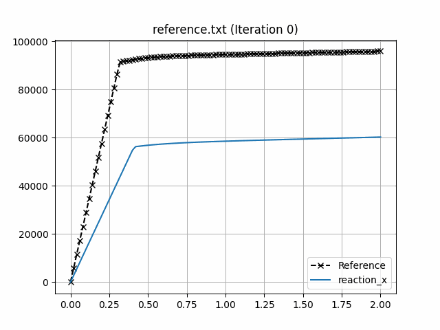
Note that despite the fact that the optimal parameters are not exactly the same as the ones used to compute the reference response, the loss function value is very small, and the fitting is excellent as can be seen in the figures below.

To visualise the optimisation results, use the piglot-plot utility. In the same directory, run (this may take a few seconds)

piglot-plot animation config.yaml

This generates an animation for all the function evaluations that have been made throughout the optimisation procedure for the two target objectives. You can find the .gif file(s) inside the output directory, which should give something like (for the minimum_value target):

Now, try running

piglot-plot parameters config.yaml

This will plot the evaluated parameters during the optimisation procedure:

To see the convergence history of the best loss function value, run

piglot-plot history config.yaml --best --log

which will generate:

To see the best-observed value for the optimisation problem, run

piglot-plot best config.yaml

which will generate:

Composite setting

This subsection aims to show the difference in the results obtained using the composite option. Convergence is more stable, a smaller loss is achieved and the parameters are closer to the reference solution.

We run 25 iterations using the botorch optimiser within the composite setting.

The configuration file (examples/abaqus_solver_fitting/config_composite.yaml) for this example is:

iters: 25

optimiser: botorch


parameters:
  Young: [100, 100, 300]
  S1: [200, 200, 400]
  S2: [500, 500, 700]


objective:
  name: fitting
  composite: True
  solver:
    name: abaqus
    # path to the Abaqus executable
    abaqus_path: C:\SIMULIA\Commands\abaqus.bat

    cases:
      'sample.inp':
        step_name: Step-1 # optional field for this case
        instance_name: Part-1-1 # optional field for this case
        fields:
          'reaction_x':
            name: FieldsOutput
            set_name: RF_SET
            field: RF
            x_field: U
            direction: x
   
  references:
    'reference.txt':
      prediction: reaction_x

The output is the following

BoTorch: 100%|███████████████████████████████████████████████████████| 25/25 [07:35<00:00, 18.24s/it, Loss: 3.4894e-10]
Completed 25 iterations in 7m35s
Best loss:  3.48943524e-10
Best parameters
- Young:   210.001758
-    S1:   324.987890
-    S2:   600.530661

The animation for all the function evaluations that have been made throughout the optimisation procedure are once again showed running

piglot-plot animation config_composite.yaml

And the output is: