Analytical curve

A simple design objective example is included to demonstrate how to use piglot in this context. In design problems, there is no reference response available, and several values of the parameters have to be evaluated for the target objectives.

In this problem, we aim to minimise the minimum value and maximimise the area below a nonlinear function given by the expression \(f(x) = |a \exp(x) + bx^2+c\sin(x)|\).

We run 10 iterations using the botorch optimiser, and set the parameters for optimisation (a, b and c) with bounds [-4,4] and initial value 0. The notation <a>, <b> and <c> indicates that these parameters should be optimised. We also define a parameterisation using the variable \(x\), where we sample the function between [-2,2] with 100 points.

The configuration file (examples/sample_curve_design/config.yaml) for this example is:

iters: 10

optimiser: botorch

parameters:
  a: [0, -4, 4]
  b: [0, -4, 4]
  c: [0, -4, 4]

objective:
  name: design
  solver:
    name: curve
    cases:
      'case_1':
        expression: abs(<a> * exp(x) + <b> * x**2 + <c> * sin(x))
        parametric: x
        bounds: [-2, 2]
        points: 100
  targets:
    'minimum_value':
      quantity: max
      prediction: ['case_1']
      negate: False
    'maximum_area':
      quantity: integral
      prediction: ['case_1']
      negate: True

The generated response with the label case_1 is optimised having two target objectives: (i) minimisation of the minimum function value minimum_value, and (ii) maximization of the area/integral below the function maximum_area.

To run this example, open a terminal inside the piglot repository, enter the examples/sample_curve_design directory and run piglot with the given configuration file

cd examples/sample_curve_design
piglot config.yaml

You should see an output similar to

BoTorch: 100%|████████████████████████████| 10/10 [00:00<00:00, 10.92it/s, Loss: -4.3239e+00]
Completed 10 iterations in 0.91609s
Best loss: -4.32393814e+00
Best parameters
- a:    -2.433969
- b:    -4.000000
- c:     4.000000

To visualise the optimisation results, use the piglot-plot utility. In the same directory, run (this may take some time)

piglot-plot animation config.yaml

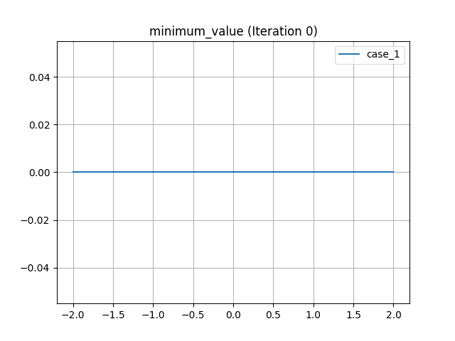
This generates an animation for all the function evaluations that have been made throughout the optimisation procedure for the two target objectives. You can find the .gif file(s) inside the output directory, which should give something like (for the minimum_value target):

Now, try running

piglot-plot parameters config.yaml

This will plot the evaluated parameters during the optimisation procedure:

To see the convergence history of the best loss function value, run

piglot-plot history config.yaml --best

which will generate: